Featured

Published on February 16th, 2023 📆 | 6573 Views ⚑

0

Definitive Dossier of Devilish Debug Details – Part Deux: A Didactic Deep Dive into Data Driven Deductions

iSpeech

In Part
One of this blog series, Steve Miller outlined what PDB paths
are, how they appear in malware, how we use them to detect malicious
files, and how we sometimes use them to make associations about groups
and actors.

As Steve continued his research into PDB paths, we became interested
in applying more general statistical analysis. The PDB path as an
artifact poses an intriguing use case for a couple of reasons.

­First, the PDB artifact is not directly tied to the functionality
of the binary. As a byproduct of the compilation process, it contains
information about the development environment, and by proxy, the
malware author themselves. Rarely do we encounter static malware
features with such an interesting tie to the human behind the
keyboard, rather than the functionality of the file.

Second, file paths are an incredibly complex artifact with many
different possible encodings. We had personally been dying to find an
excuse to spend more time figuring out how to parse and encode paths
in a more useful way. This presented an opportunity to dive into this
space and test different approaches to representing file paths in
various models.

The objectives of our project were:

1. Build a large data set of PDB paths and apply some statistical
   methods to find potentially new signature terms and logic.
2. Investigate whether applying machine learning classification
   approaches to this problem could improve our detection above writing
   hand-crafted signatures.
3. Build a PDB classifier as a weak
   signal for binary analysis.

To start, we began gathering data. Our dataset, pulled from internal
and external sources, started with over 200,000 samples. Once we
deduplicated by PDB path, we had around 50,000 samples. Next, we
needed to consistently label these samples, so we considered various
labeling schemes.

Labeling Binaries With PDB Paths

For many of the binaries we had internal FireEye labels, and for
others we looked up hashes on VirusTotal (VT) to have a look at their
detection rates. This covered the majority of our samples. For a
relatively small subset we had disagreements between our internal
engine and VT results, which merited a slightly more nuanced policy.
The disagreement was most often that our internal assessment
determined a file to be benign, but the VT results showed a nonzero
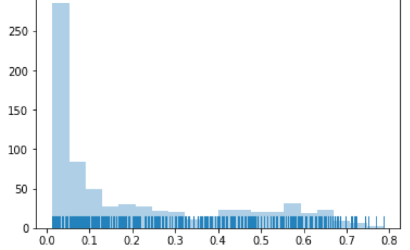
percentage of vendors detecting the file as malicious. In these cases
we plotted the ‘VT ratio”: that is, the percentage of vendors labeling
the files as malicious (Figure 1).

Figure 1: Ratio of vendors calling file
bad/total number of vendors

The vast majority of these samples had VT detection ratios below
0.3, and in those cases we labeled the binaries as benign. For the
remainder of samples we tried two strategies – marking them all as
malicious, or removing them from the training set entirely. Our
classification performance did not change much between these two
policies, so in the end we scrapped the remainder of the samples to
reduce label noise.

Building Features

Next, we had to start building features. This is where the fun
began. Looking at dozens and dozens of PDB paths, we simply started
recording various things that ‘pop out’ to an analyst. As noted
earlier, a file path contains tons of implicit information, beyond
simply being a string-based artifact. Some analogies we have found
useful is that a file path is more akin to a geographical location in
its representation of a location on the file system, or like a
sentence in that it reflects a series of dependent items.

To further illustrate this point, consider a simple file path such as:

C:UsersWorldDesktopduckZbw138ht2aeja2.pdb (source file)

This path tells us several things:

• This software was compiled on the system drive of the
  computer
• In a user profile, under user ‘World’
• The
  project is managed on the Desktop, in a folder called ‘duck’
• The filename has a high degree of entropy and is not very easy
  to remember

In contrast, consider something such as:

D:VSCORE5BUILDVSCorereleaseEntVUtil.pdb
(source file)

This indicates:

• Compilation on an external or secondary drive
• Within
  a non-user directory
• Contains development terms such as
  ‘BUILD’ and ‘release’
• With a sensible, semi-memorable file
  name

These differences seem relatively straightforward and make intuitive
sense as to why one might be representative of malware development
whereas the other represents a more “legitimate-looking” development environment.

Feature Representations

How do we represent these differences to a model? The easiest and
most obvious option is to calculate some statistics on each path.
Features such as folder depth, path length, entropy, and counting
things such as numbers, letters, and special characters in the PDB
filename are easy to compute.

However, upon evaluation against our dataset, these features did not
help to separate the classes very well. The following are some
graphics detailing the distributions of these features between our
classes of malicious and benign samples:

While there is potentially some separation between benign and
malicious distributions, these features alone would likely not lead to
an effective classifier (we tried). Additionally, we couldn’t easily
translate these differences into explicit detection rules. There was
more information in the paths that we needed to extract, so we began
to look at how to encode the directory names themselves.

Normalization

As with any dataset, we had to undertake some steps to normalize the
paths. For example, the occurrence of individual usernames, while
perhaps interesting from an intelligence perspective, would be
represented as distinct entities when in fact they have the same
semantic meaning. Thus, we had to detect and replace usernames
with to normalize this representation. Other folder
idiosyncrasies such as version numbers or randomly generated
directories could similarly be normalized into or .

A typical normalized path might therefore go from this:

C:UsersjsmithDocumentsVisual Studio 2013Projectsmkzyu91952mkzyu91952objx86Debugmkzyu91952.pdb

To this:

c:usersdocumentsvisual studio 2013projectsobjx86debugmkzyu91952.pdb

You may notice that the PDB filename itself was not normalized. In
this case we wanted to derive features from the filename itself, so we
left it. Other approaches could be to normalize it, or even to make
note that the same filename string ‘mkzyu91952’ appears earlier in the
path. There are endless possible features when dealing with file paths.

Directory Analysis

Once we had normalized directories, we could start to “tokenize”
each directory term, to start performing some statistical
analysis. Our main goal of this analysis was to see if there were any
directory terms that highly corresponded to maliciousness, or see if
there were any simple combinations, such as pairs or triplets, that
exhibited similar behavior.

We did not find any single directory name that easily separated the
classes. That would be too easy. However, we did find some general
correlations with directories such as “Desktop” being somewhat more
likely to be malicious, and use of shared drives such as Z: to be more
indicative of a benign file. This makes intuitive sense given the more
collaborative environment a “legitimate” software development process
might require. There are, of course, many exceptions and this is what
makes the problem tricky.

Another strong signal we found, at least in our dataset, is that
when the word “Desktop” was in a non-English language and particularly
in a different alphabet, the likelihood of that PDB path being tied to
a malicious file was very high (Figure 2). While potentially useful,
this can be indicative of geographical bias in our dataset, and
further research would need to be done to see if this type of
signature would generalize.

Figure 2: Unicode desktop folders from
malicious samples

Various Tokenizing Schemes

In recording the directories of a file path, there are several ways
you can represent the path. Let’s use this path to illustrate these
different approaches:

c:LeavesmellLongruleThis.pdb (file)

Bag of Words

One very simple way is the “bag-of-words”
approach, which simply treats the path as the distinct set of
directory names it contains. Therefore, the aforementioned path would
be represented as:

[‘c:’,’leave’,’smell’,’long’,’rulethis’]

Positional Analysis

Another approach we considered was recording the position of each
directory name, as a distance from the drive. This retained more
information about depth, such that a ‘build’ directory on the desktop
would be treated differently than a ‘build’ directory nine directories
further down. For this purpose, we excluded the drives since they
would always have the same depth.

[’leave_1’,’smell_2’,’long_3’,’rulethis_4’]

N-Gram Analysis

Finally, we explored breaking paths into n-grams; that is, as a
distinct set of n- adjacent directories. For example, a 2-gram
representation of this path might look like:

[‘c:leave’,’leavesmell’,’smelllong’,’longrulethis’]

We tested each of these approaches and while positional analysis and
n-grams contained more information, in the end, bag-of-words
seemed to generalize best. Additionally, using the bag-of-words
approach made it easier to extract simple signature logic from the
resultant models, as will be shown in a later section.

Term Co-Occurrence

Since we had the bag-of-words vectors created for each path, we were
also able to evaluate term co-occurrence across benign and malicious
files. When we evaluated the co-occurrence of pairs of terms, we found
some other interesting pairings that indeed paint two very different
pictures of development environments (Figure 3).

Figure 3: Correlated pairs with malicious and
benign files

Keyword Lists

Our bag-of-words representation of the PDB paths then gave us a
distinct set of nearly 70,000 distinct terms. The vast majority of
these terms occurred once or twice in the entire dataset, resulting in
what is known as a ‘long-tailed’ distribution. Figure 4 is a graph of
only the top 100 most common terms in descending order.

Figure 4: Long tailed distribution of
term occurrence

As you can see, the counts drop off quickly, and you are left
dealing with an enormous amount of terms that may only appear a
handful of times. One very simple way to solve this problem, without
losing a ton of information, is to simply cut off a keyword list after
a certain number of entries. For example, take the top 50 occurring
folder names (across both good and bad files), and save them as a
keyword list. Then match this list against every path in the dataset.
To create features, one-hot
encode each match.  

Rather than arbitrarily setting a cutoff, we wanted to know a bit
more about the distribution and understand where might be a good place
to set a limit – such that we would cover enough of the samples
without drastically increasing the number of features for our model.
We therefore calculated the cumulative number of samples covered by
each term, as we iterated down the list from most common to least
common. Figure 5 is a graph showing the result.

Figure 5: Cumulative share of samples
covered by distinct terms

As you can see, with only a small fraction of the terms, we can
arrive at a significant percentage of the cumulative total PDB paths.
Setting a simple cutoff at about 70% of the dataset resulted in
roughly 230 terms for our total vocabulary. This gave us enough
information about the dataset without blowing up our model with too
many features (and therefore, dimensions). One-hot encoding the
presence of these terms was then the final step in featurizing the
directory names present in the paths.

YARA Signatures Do Grow on Trees

Armed with some statistical features, as well as one-hot encoded
keyword matches, we began to train some models on our now-featurized
dataset. In doing so, we hoped to use the model training and
evaluation process to give us insights into how to build better
signatures. If we developed an effective classification model, that
would be an added benefit.

We felt that tree-based models made sense for this use case for two
reasons. First, tree-based models have worked well in the past in
domains requiring a certain amount of interpretability and using a
blend of quantitative and categorical features. Second, the features
we used are largely things we could represent in a YARA signature.
Therefore, if our models built boolean logic branches that separated
large numbers of PDB files, we could potentially translate these into
signatures. This is not to say that other model families could not be
used to build strong classifiers. Many other options ranging from Logistic
Regression to Deep Learning
could be considered.

We fed our featurized training set into a Decision
Tree, having set a couple ‘hyperparameters’ such as max depth and
minimum samples per leaf, etc. We were also able to use a sliding
scale of these hyperparameters to dynamically create trees and,
essentially, see what shook out. Examining a trained decision tree
such as the one in Figure 6 allowed us to immediately build new signatures.

Figure 6: Example decision tree and
decision paths

We found several other interesting tidbits within our decision
trees. Some terms that resulted in completely or almost-completely
malicious subgroups are:

We also found the term ‘WindowsApplication1’ to be quite useful. 89%
of the files in our dataset containing this directory were malicious.
Cursory research indicates that this is the default directory
generated when using Visual Studio to compile a Windows binary. Once
again, this makes some intuitive sense for finding malware authors.
Training and evaluating decision trees with various parameters turned
out to be a hugely productive exercise in discovering potential new
signature terms and logic.

Classification Accuracy and Findings

Since we now had a large dataset of PDB paths and features, we
wanted to see if we could train a traditional classifier to separate
good files from bad. Using a Random Forest
with some tuning, we were able to achieve an average accuracy of 87%
over 10 cross validations. However, while our recall (the percentage
of bad things we could identify with the model) was relatively high at
89%, our malware precision (the share of those things we called bad
that were actually bad) was far too low, hovering at or below 50%.
This indicates that using this model alone for malware detection would
result in an unacceptably large number of false positives, were we to
deploy it in the wild as a singular detection platform. However, used
in conjunction with other tools, this could be a useful weak signal to
assist with analysis.

Conclusion and Next Steps

While our journey of statistical PDB analysis did not yield a magic
malware classifier, it did yield a number of useful findings that we
were hoping for:

1. We developed several file path feature functions which are
   transferable to other models under development.
2. By diving
   into statistical analysis of the dataset, we were able to identify
   new keywords and logic branches to include in YARA signatures. These
   signatures have since been deployed and discovered new malware
   samples.
3. We answered a number of our own general research
   questions about PDB paths, and were able to dispel some theories we
   had not fully tested with data.

While building an independent classifier was not the primary goal,
improvements can surely be made to improve the end model accuracy.
Generating an even larger, more diverse dataset would likely make the
biggest impact on our accuracy, recall, and precision. Further
hyperparameter tuning and feature engineering could also help. There
is a large amount of established research into text classification
using various deep learning methods such as LSTMs,
which could be applied effectively to a larger dataset.

PDB paths are only one small family of file paths that we encounter
in the field of cyber security. Whether in initial infection, staging,
or another part of the attack lifecycle, the file paths found during
forensic analysis can reveal incredibly useful information about
adversary activity. We look forward to further community research on
how to properly extract and represent that information.

Source link

Tagged with: data • debug • deductions • definitive • details • deux • devilish • didactic • DidacticDeep • Dive • dossier • driven • Part