Conjunction And Disruption: Technology, War, And Asset Prices – Part 1

For the last year, and especially the last six months, I have been writing a great deal about the likelihood of a long-term downturn in the market led by the tech sector. This argument is built primarily on the notion of long-term mean reversions at the level of the market as a whole (in both price and earnings growth) and in a total rebalancing of sectors (away from tech and towards cyclicals) triggered by a commodity shock. In other words, the behavior of the stock market at both the overall and sectoral levels, as well as commodity behavior, suggest both a reversal in the sectoral hierarchy of the last decade and a substantial growth shock. Here are some of those articles:

Needless to say, disagreement is unavoidable, since there is so much that we do not know about how and why markets behave the way they do. When it comes to technology, those disagreements seem to fall into three classes which often overlap.

First, nobody can predict the future.

Second, the future, especially in the technology sector, is unstoppable.

Third, a particular favorite (entrepreneur, company, industry, technology) is unstoppable.

The first argument is often deployed primarily as a way of running interference for one or both of the two subsequent claims. First, they disarm you by pointing out that the future is unknowable. Now that you are defenseless, they remind you of how powerful the performance of technology both in real terms (that is, actual new innovations) and financial terms (market performance) has been, and then they point out that new innovations will continue to be produced (again, in a particular sector, industry, or company, or by a particular entrepreneur).

The problem is, even if one agreed with all of these statements, the conclusion that these forces will be reflected in equity prices is contrary to both the history and theory of the relationship between innovation and market performance. For this series, I have scanned the history of innovation of the last 200 years and compared that to both market performance and social stability, and I have found some pretty strong relationships. These relationships, with a little bit of updating, seem to confirm the central arguments of the “prophet of innovation,” the master of “creative destruction,” Joseph Schumpeter, about innovation and markets. They also confirm the central observations of the Copernicus of economics, Nikolai Kondratiev, who inspired Schumpeter’s theory of innovation. It also suggests that neither Schumpeter nor Kondratiev can be understood apart from one another, although partisans of each thinker regularly sever or downplay the links between the two. In fact, if the bulk of my argument is correct, I think a good case could be made for their deserving posthumous awards for the Nobel Prize, particularly in the case of Kondratiev, who appears to have been one of the few people ever killed for their strictly economic beliefs. What the ultimate legacy of these two Eastern Europeans ought to be is a question for a different occasion, however. Here, we are primarily concerned with establishing what the relationship between innovation and markets is.

In this series, I intend to argue the following points about the interactions between technology, war, and financial markets:

1. Financial markets

• Real commodity prices and the earnings yield rise and fall together
• Real stock prices rise and fall with the EPS/commodity ratio
• Cycles in prices and yields seem to be more or less regular (50-60 years under the gold standard and 30 years under a fiat standard)
• Under a fiat monetary standard, secular bull markets in equities tend to occur as yields fall
• Real commodity prices and equity yields have remained near historic lows over the last 30 years

2. War

• Deaths in political conflict seem to rise and fall in sympathy with real commodity prices and the earnings yield
• Major conflicts seem to be more or less regular (peaking every 50-60 years prior to World War I and peaking every 30 years since World War I)
• Deaths in political conflict have been at their lowest ebb since the late 19^th century

3. Technology

• The mass diffusion of significant innovations occurs primarily during secular declines in yields, commodity prices, and global political violence
• Peaks in frequency curves for significant innovations occur primarily during secular declines in yields, commodity prices, and global political violence
• The initial diffusion of significant innovations occurs primarily during secular rises in yields, commodity prices, and global political violence
• From the introduction of an innovation to its ubiquity, the growth rate in the rate of diffusion declines almost continuously but declines most precipitously when the innovation passes from initial diffusion to mass diffusion, apparently at the moment of diffusion “take-off”
• Differentiations occur during the period of mass diffusion; this is in contrast to the period of standardization that occurs during the period of initial diffusion

Let me try to squeeze as much of this as I can into a handful of charts. In the charts below, “K Waves” is an abstraction representing real commodity prices, equity yields, and global deaths in conflicts. Juxtaposed to those waves in prices, yields, and deaths in conflicts are innovation waves expressed in terms of the diffusion of disruptive goods.

The first chart, for example, shows that growth in the diffusion of disruptive innovations is highest during rising Kondratiev waves (rising commodity prices, rising yields, and rising violence). As this wave of commodity inflation, high yields, and violence crests, growth rates in the diffusion of these disruptive innovations—incidentally, this also appears to be true for sales growth, as well—suddenly drop off. As inflation, yields, and violence subsides, these disruptive innovations quickly become ubiquitous.

The following chart draws out the relationship between the idealized “K Wave” (in yellow), the growth rate in diffusion (in orange) and the frequency curve (in grey). The “frequency curve” is simply the difference between the diffusion rate of a given period and that of the previous period; it performs as something like a proxy for sales. The relationship between the growth rate and the frequency curve is somewhat analogous to the relationship between the initial growth rate and the terminal value, respectively, in a two-stage DCF model.

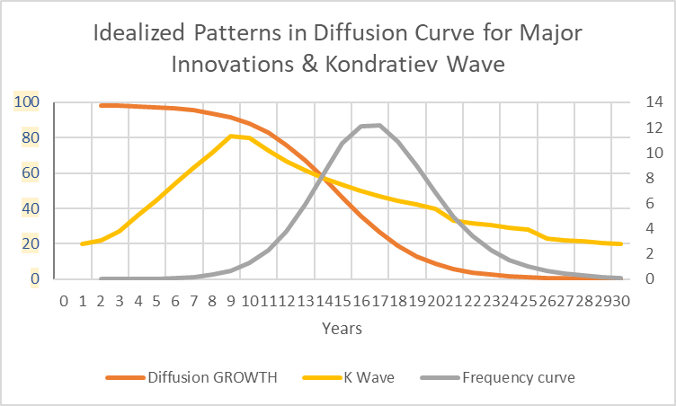
So, Chart B is Chart A without the diffusion curve. In Chart C, we add the diffusion curve back in, take out the K Wave and add in the stock market in a normal fiat scenario.

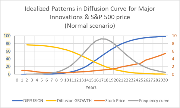
Notice that stocks tend to fall while the growth rate in the disruptive innovation wave is high. Prices rise as growth falls and the frequency curve mounts, and prices continue to rise even as the market nears saturation.

In the following chart, I compare the K Wave to stock prices and earnings per share (EPS) under a normal fiat scenario.

Earnings growth remains high and constant, but prices fall as commodity prices, yields, and violence rise.

In the following chart, I show an alternative scenario that occurred once in the last century.

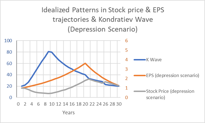
In the 1930s, earnings collapsed about halfway through the decline in the K Wave.

One problem with these idealized representations is that they smooth out the volatility that tends to occur along the way, and as I have tried to show in the articles I linked to at the beginning, cyclical volatility contains important information about long-term performance. In this chart, earnings are presented as in more or less steady decline for a decade.

Chart F is the same as Chart E, but it includes a value for “technology” that grows at a steady rate.

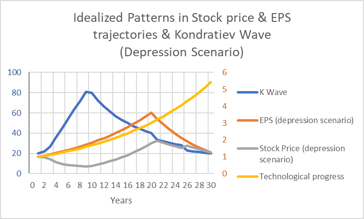
In other words, these relationships seem to hold true even where the underlying rate of technological growth seems to remain constant. Although it might be absurd to say that disruptive innovation waves occur independently of technological growth, technological growth and disruptive innovation are not the same thing. An analogy might be evolution, where selective pressure is (presumably) constant yet the geologic record suggests punctuated equilibrium is the rule. Or, we might think of these disruptive innovation waves as miniature paradigm shifts. We do not need to be too fancy about this, however. An analogy from daily life could be consistently working on a skill of some kind and finding that the progress appears to be manifested as periodic, epiphanous breakthroughs along the way.

The most obvious example of steady technological growth is Moore’s Law, which has grown at an annual rate of 41% for the last 50 years.

By my reckoning, we have been through two innovation waves since the beginning of this chart in 1970, but this is not to be found in the behavior of Moore’s Law (so far as I can tell).

Of course, I can plot as many idealized charts as I like, but the question is whether or not they resemble reality or not. In subsequent installments in this series, I am going to go through the diffusion of automobiles, radios, televisions, personal computers, and smartphones, as well as secondary innovations like refrigerators, washing machines, VCRs, toilets, and air travel to try to prove that this is the case.

But let’s take a look at railroads for a moment, first. The following chart shows the diffusion of railroad mileage in the US from 1830 to 1950.

According to the points listed earlier in the article, the primary diffusion of a disruptive innovation should occur during a decline in prices and yield. The best way to measure surges in diffusion is via the frequency curve, which is represented by miles of railroad built per decade (in grey). The Kondratiev peak (the peak in commodities, yields, and conflict deaths) should occur at the transition from a high-growth/low-diffusion stage to a low-growth/high diffusion stage.

The following chart is composed of the two primary elements of Kondratiev waves, commodity prices and yields. I calculated commodity prices as a geometric average of coal, copper, cotton, and wheat prices. A peak in commodity prices, yields, and global deaths in conflicts are typical of Kondratiev peaks, so the peak we are primarily concerned with is the one in the 1860s. In terms of conflict, the 1860s were marked by extremely bloody local and regional wars on virtually every continent.

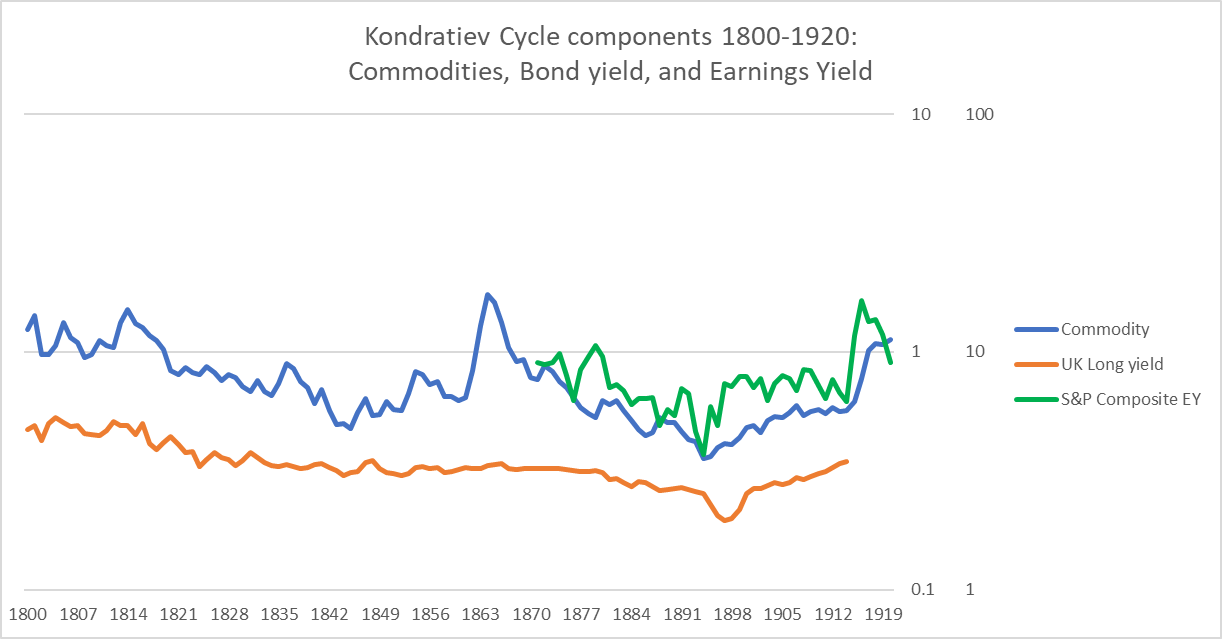
It is clear that the diffusion of the railroad primarily occurred during the period after the 1860s, but rail technology’s highest growth period was prior to that decade. That pattern of growth is typical of logistic diffusion curves; they start off with very high growth rates which decelerate more or less consistently over time. As I discovered while writing this, the easiest way to create a logistic curve is simply by taking an initial growth rate and then multiplying it by some constant value between 0 and 1 (for example, if period 1 has 100% growth and each subsequent rate of growth is 90% of the previous period’s, that would produce growth rates of 90% for period 2, 81% for period 3, etc.). In other words, these growth rates fall in a largely logarithmic fashion.

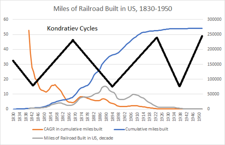
As someone who is not good with math, I found this interesting, frustrating, and ultimately distracting. The point is less where that precise transition from high-growth/low-diffusion to low-growth/high-diffusion occurs than that these disruptive innovations typically catch fire during the rising period of Kondratiev cycles and then “disrupt” society by spreading to every nook and cranny during the downswing. In fact, one of the big questions worth considering along the way is, which is more disruptive, the period of high growth or high diffusion? And, what is it precisely that is being disrupted? The technological world? Particular classes of products? Some asset classes but not others? The economy generally? Geopolitical order? Social dynamics? Human perception? And, is it a one-way street? If technology is impacting long-term market behavior and geopolitical order, are those two feeding back into the way innovation evolves?

I think the answer is Yes to most of these questions. In the following chart, I have drawn another idealized version of Kondratiev waves and their expression at the level of technology and innovation. I hope it can act as a springboard to thinking about the way innovations erupt into the social organism (markets, politics, society). There is often a period of abstract developments occurring within a particular technology/innovation/social regime (e.g., bicycles, buggies, streetcars, urbanization, modernization) that coagulate into inventions (say, cars); those inventions are then refined by innovators who are able to bring them to market (Henry Ford, for example). Those innovation periods have been relatively rapid in the last century, and by the time the Kondratiev cycle has topped out, the innovation has grabbed a toehold in the market that it will not let go. That does not mean that the innovation will not undergo further improvements (for example, GM made improvements to cars on multiple axes during the 1920s). But, no sooner is mass diffusion underway than new technologies and new innovations are gestating in preparation for the next cycle.

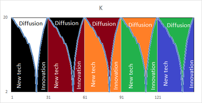
As we go along, I think we will find that there are plenty of reasons to be dissatisfied with this portrayal of the innovation dynamics, but I found it especially helpful when thinking about which point is most likely to be disruptive and to whom or what it might be causing disruptions.

Ultimately, we will bring this back to how we can read these cycles in real time and what their implications are for investors. What is clear to me from this historical research is that stock markets, even technology stocks, should not be treated as simple proxies for Technology, Progress, and Innovation. Even during periods of roaring technological growth and innovation, these markets can perform horribly. Over the very long term, investors have to judge how that technological growth makes its way into markets through earnings and price.

Comments are closed.